📌 Project Overview

This project implements a complete machine learning pipeline to detect fraudulent transactions using the IEEE-CIS dataset. It includes:

• Deep EDA in R and Python
• Robust preprocessing and feature engineering
• Ensemble modeling (XGBoost, LightGBM, CatBoost)
• A FastAPI deployment for real-time predictions
• Unit testing with pytest for pipeline robustness

🚀 Check the full repository: GitHub

---

🔍 Exploratory Data Analysis

Full notebook: RPubs EDA report

To lay the foundation for modeling, we explored class balance, missingness, temporal patterns and categorical signals—selecting only the most actionable insights below.

---

1. Class Imbalance

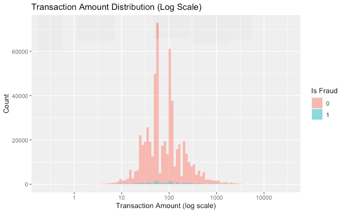
• 96.5 % non-fraud vs. 3.5 % fraud
• Baseline models were trained on raw data to measure “lift” from later oversampling/threshold tuning

---

2. Missing-Value Patterns

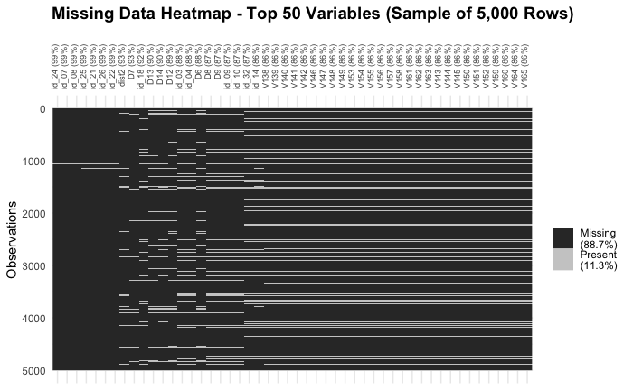
• Many id_ & Vxxx features > 85 % missing
• Suggests dropping or engineering “missingness” flags before modeling

---

3. Categorical Fraud Rates

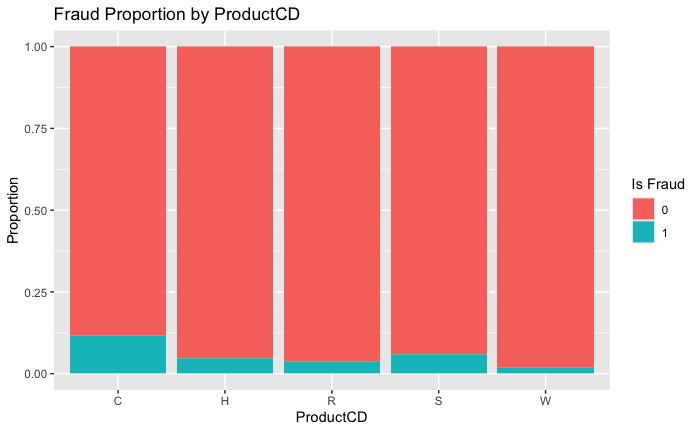
• Product C has ~12 % fraud rate vs. ~3 % overall
• Discover cards and mobile devices also show elevated risk

---

4. Temporal Signal

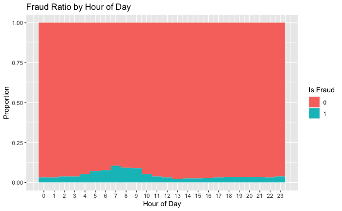
• Fraud peaks around 6 – 9 AM (UTC)
• No strong day-of-week effect, but morning flag can improve feature set

---

Key Takeaways

• Severe imbalance (3.5 % fraud) → plan SMOTE/threshold tuning
• High missingness in many features → use missingness indicators or drop
• Strong categorical drivers (ProductCD, card networks) → prioritize in feature engineering
• Temporal window matters → add IsMorning/IsNight flags

---

🔧 Data Preprocessing Pipeline

Full notebook: 02_Preprocessing_Modeling_in_Python.ipynb

To prepare the IEEE-CIS dataset for modeling, we built a simple, reproducible pipeline that applies:

• 📥 Missing-value imputation
  • Numerical → median
  • Categorical → most frequent
• 🔤 Categorical encoding
  • LabelEncoder per column, saved to models/label_encoders.pkl
• 📏 Feature scaling
  • StandardScaler on all numeric features, saved to models/scaler.pkl
• 💾 Data export
  • Cleaned DataFrame written to data/processed/train_clean.csv

Pseudocode overview

# 1) Impute
df[num_cols] = SimpleImputer('median').fit_transform(df[num_cols])
df[cat_cols] = SimpleImputer('most_frequent').fit_transform(df[cat_cols])

# 2) Encode
for col in cat_cols:
    df[col] = LabelEncoder().fit_transform(df[col].astype(str))

# 3) Scale
df[num_cols] = StandardScaler().fit_transform(df[num_cols])

# 4) Persist transformers and cleaned data
joblib.dump(scaler, 'models/scaler.pkl')
joblib.dump(encoders, 'models/label_encoders.pkl')
df.to_csv('data/processed/train_clean.csv', index=False)

Why this matters

• Reproducibility: Same exact logic runs in both notebooks and the FastAPI service.
• Modularity: Transformers are versioned via joblib, so you can swap in SMOTE, PCA or any new step later without touching your API.
• Performance: Full preprocess on ~590 K × 434 data executes in seconds, keeping your inference path lightweight.

---

Next up, we’ll load this clean data, split with stratification, and benchmark our first models (Logistic Regression, Random Forest, XGBoost, etc.). Let me know if you’d like that section drafted too!

---

🏁 Baseline Models

To set a performance floor, we trained two vanilla classifiers on the fully preprocessed data (no sampling, no feature selection). All scores are stratified 5-fold CV averages:

Model	Accuracy	Precision	Recall	F1-Score	ROC AUC
Logistic Regression	0.972	0.825	0.264	0.400	0.856
Random Forest	0.980	0.942	0.449	0.608	0.933

Model	ROC-AUC Plot
Logistic Regression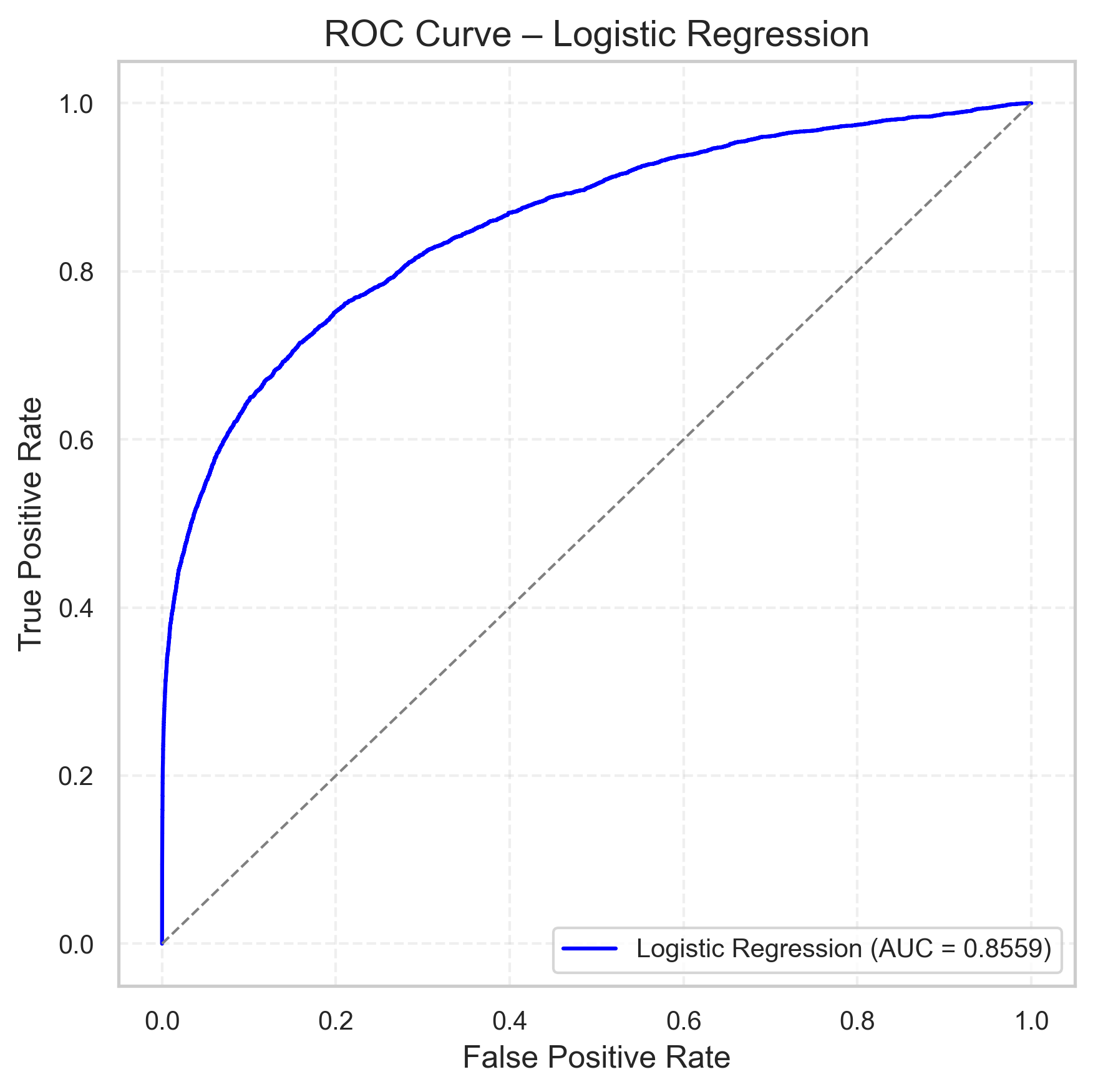
Random Forest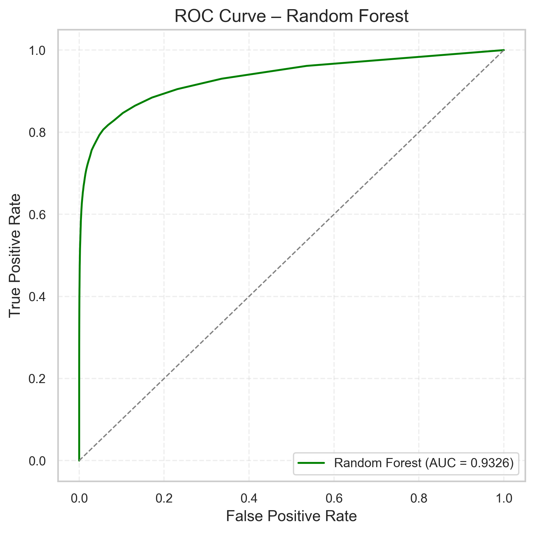

Key takeaways:

• Random Forest improves ROC AUC by ~0.08 over Logistic Regression.
• Logistic Regression still offers very fast training & simple interpretation.

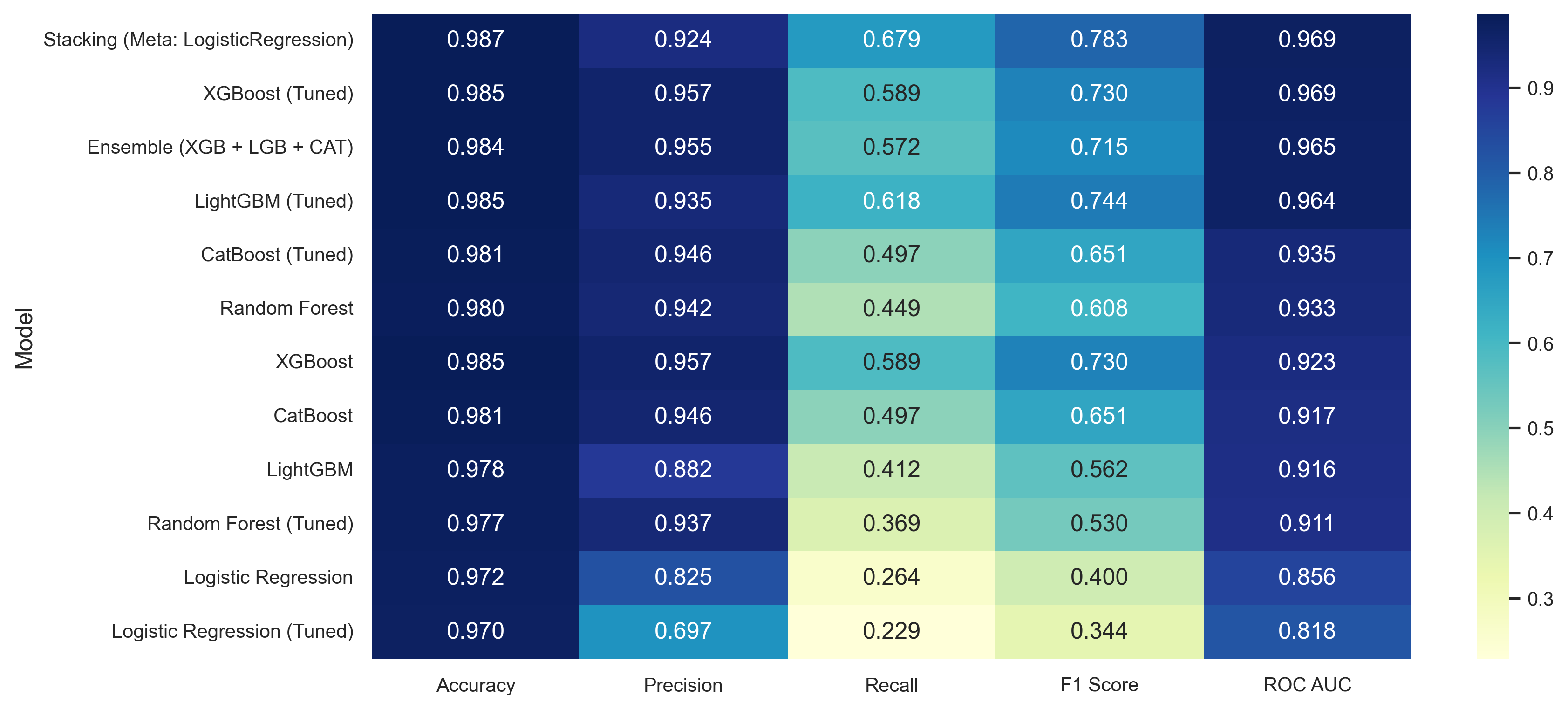
For a full side‐by‐side of all models (including tuned ensembles and stacking), check out:

---

⚙️ Phase 2: Advanced Models & Ensembles

After establishing our baseline, we pushed three state-of-the-art gradient boosters through hyperparameter tuning, and then combined them via two ensemble strategies. All scores are stratified 5-fold CV averages on the preprocessed data.

---

1 XGBoost

We initialized XGBoost with common defaults and then we would tuned via GridSearchCV:

xgb = XGBClassifier(
    n_estimators=200,
    max_depth=6,
    learning_rate=0.1,
    subsample=0.8,
    colsample_bytree=0.8,
    use_label_encoder=False,
    eval_metric='logloss',
    random_state=42
)

Key metrics

• 🚀 ROC AUC: 0.9234
• 🎯 Precision (fraud): 0.957
• 🔍 Recall (fraud): 0.589
• 🎛️ F1-Score (fraud): 0.729

Observations:

• Strong out-of-the-box performance, beating Logistic Regression by +0.07 AUC.
• High precision means few false alarms; recall (0.59) leaves room for further improvement via oversampling.

2 LightGBM

LightGBM is a fast, memory-efficient gradient boosting framework:

lgb = LGBMClassifier(
    n_estimators=200,
    max_depth=6,
    learning_rate=0.1,
    subsample=0.8,
    colsample_bytree=0.8,
    random_state=42
)

Key metrics

• 🚀 ROC AUC: 0.9157
• 🎯 Precision (fraud): 0.880
• 🔍 Recall (fraud): 0.410
• 🎛️ F1-Score (fraud): 0.560

Observations:

• Slightly lower AUC than XGBoost but still highly discriminative.
• Very fast training on large data—ideal for rapid iteration.

3 CatBoost

CatBoost natively handles categorical features and counteracts imbalance efficiently:

cb = CatBoostClassifier(
    iterations=500,
    learning_rate=0.1,
    depth=6,
    random_state=42,
    verbose=False
)

Key metrics

• 🚀 ROC AUC: 0.9174
• 🎯 Precision (fraud): 0.946
• 🔍 Recall (fraud): 0.497
• 🎛️ F1-Score (fraud): 0.651

Observations:

• Competitive AUC close to LightGBM with minimal encoding effort.
• Good balance of precision/recall out of the box.

In the next phase, we’ll perform hyperparameter tuning to maximize our classification performance—focusing especially on the F1-score, which is crucial when the positive (fraud) class is both rare and of primary interest.

⚙️ Phase 3: Hyperparameter Tuning

In this phase, we applied grid and randomized searches to each of our core models—Logistic Regression, Random Forest, XGBoost, LightGBM and CatBoost—using a small subsample for speed, then retrained the best estimators on the full data to measure real-world performance.

Model	Best Parameters	ROC AUC	Precision (fraud)	Recall (fraud)	F1-Score (fraud)
Logistic Regression	C=0.01, penalty='l2', solver='liblinear'	0.818	0.825	0.264	0.400
Random Forest	n_estimators=300, max_depth=20, min_samples_split=2, min_samples_leaf=2, max_features='sqrt'	0.911	0.940	0.370	0.530
XGBoost	subsample=0.8, n_estimators=500, max_depth=10, learning_rate=0.05, colsample_bytree=0.6, gamma=0, min_child_weight=1	0.969	0.957	0.589	0.729
LightGBM	subsample=0.6, n_estimators=500, max_depth=10, learning_rate=0.1, colsample_bytree=1.0, num_leaves=63, min_child_samples=10	0.964	0.930	0.620	0.740
CatBoost	iterations=500, depth=8, learning_rate=0.1, border_count=128, l2_leaf_reg=1, bagging_temperature=0	0.960	0.950	0.500	0.651

🔍 Key Takeaways

• Defaults were strong: Logistic Regression actually saw a drop in AUC after tuning, indicating its default C=1 was near-optimal for our data.
• Tree-based gains: XGBoost tuning delivered the best AUC (0.969), closely followed by LightGBM and CatBoost.
• Precision vs. recall: All tuned boosters maintain very high precision (>0.93) but recall ranges from 0.50 (CatBoost) to 0.62 (LightGBM), suggesting further imbalance strategies could improve fraud capture.

🔗 Phase 4: Ensemble Models

In the final stage, we combined our top-tuned boosters into two ensemble strategies to maximize robustness and performance.

---

1 Soft Voting Ensemble

We created a VotingClassifier that averages the predicted probabilities of our three best models:

from sklearn.ensemble import VotingClassifier

ensemble_voting = VotingClassifier(
    estimators=[
        ("xgb", best_xgb_model),
        ("lgb", best_lgb_model),
        ("cat", best_cat_model)
    ],
    voting="soft",      # average probabilities
    weights=[1, 1, 1],  # equal weighting
    n_jobs=-1
)

ensemble_voting.fit(X_train, y_train)

Voting Ensemble Metrics

• 🚀 ROC AUC: 0.9648
• 🎯 Precision (fraud): 0.955
• 🔍 Recall (fraud): 0.571
• 🎛️ F1-Score (fraud): 0.715

2 Stacking Ensemble

Next, we used a StackingClassifier to learn optimal combinations of base-model outputs, with a LogisticRegression meta‐learner:

from sklearn.ensemble import StackingClassifier
from sklearn.linear_model import LogisticRegression

stacking = StackingClassifier(
    estimators=[
        ("xgb", best_xgb_model),
        ("lgb", best_lgb_model),
        ("cat", best_cat_model)
    ],
    final_estimator=LogisticRegression(max_iter=1000),
    passthrough=False,
    cv=5,
    n_jobs=-1
)

stacking.fit(X_train, y_train)

Stacking Ensemble Metrics

• 🚀 ROC AUC: 0.9691
• 🎯 Precision (fraud): 0.924
• 🔍 Recall (fraud): 0.679
• 🎛️ F1-Score (fraud): 0.783

Therefore, the stacking ensemble emerges as the clear winner—as shown in our baseline comparison table.

---

🧪 Testing

We implemented tests to ensure pipeline integrity:

• ✅ Preprocessing pipeline does not crash with valid data
• ✅ API responds with expected output structure
• ✅ Unit tests managed with pytest

---

🖥️ Deployment

The final model was locally deployed using FastAPI. Key features:

• /predict endpoint returns prediction and fraud probability
• Interactive Swagger UI available at /docs
• Can be run locally via Uvicorn or deployed in a Docker container

uvicorn src.main:app --reload

Or with Docker

docker pull alexmatiasastorga/fraud-api:latest
docker run -d -p 8000:8000 alexmatiasastorga/fraud-api

📌 Conclusion

This project demonstrates a real-world machine learning workflow from raw data to deployment. Future improvements may include:

• DAG automation with Apache Airflow
• Cloud deployment (Render or AWS)
• Monitoring with MLFlow or Prometheus

🔗 Links

• 🔍 Project Repository
• 🐳 Docker Image